Creating a Database via Webscraping from ANBIMA [R]
In this post, I will teach how to create a webscraping script with R and how to automate its execution using Windows task scheduler. This way, we will have a .csv file that receives new data at each weekly execution.
TABLE OF CONTENTS
- Why capture this data?
- What is this data and what is it used for?
- Creating the R Script
- Scheduling the script execution
1 - Why capture this data?
ANBIMA makes the daily estimation of the term structure of interest rates (ETTJ) available on this page, but the site only allows access to data from the last 5 business days.
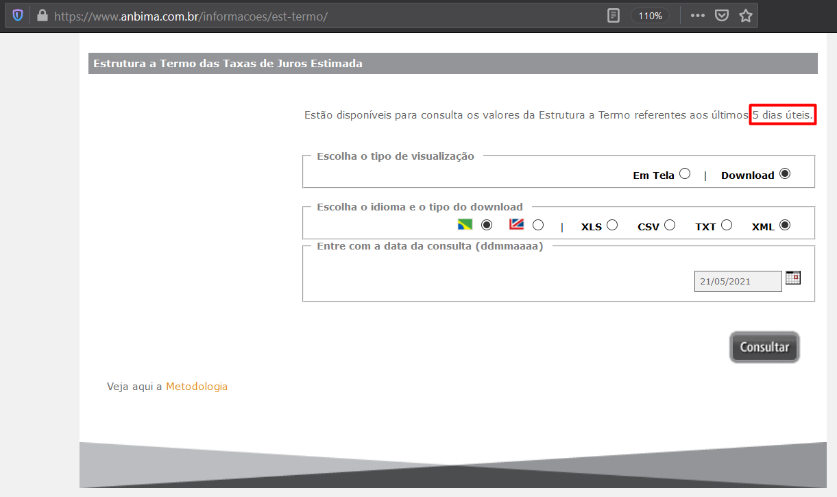 Since not everyone has a Bloomberg terminal to access this daily data, I decided to create my own database using a script that runs weekly.
2 - What is this data and what is it used for?
The daily estimation of the Term Structure of Interest Rates (ETTJ) is done using the yield curve parameters made available by ANBIMA. With this data (model parameters), it is possible to generate different yield curves for my fixed income scenario analyses. Below is an example of a comparative analysis of yield curves between two periods.
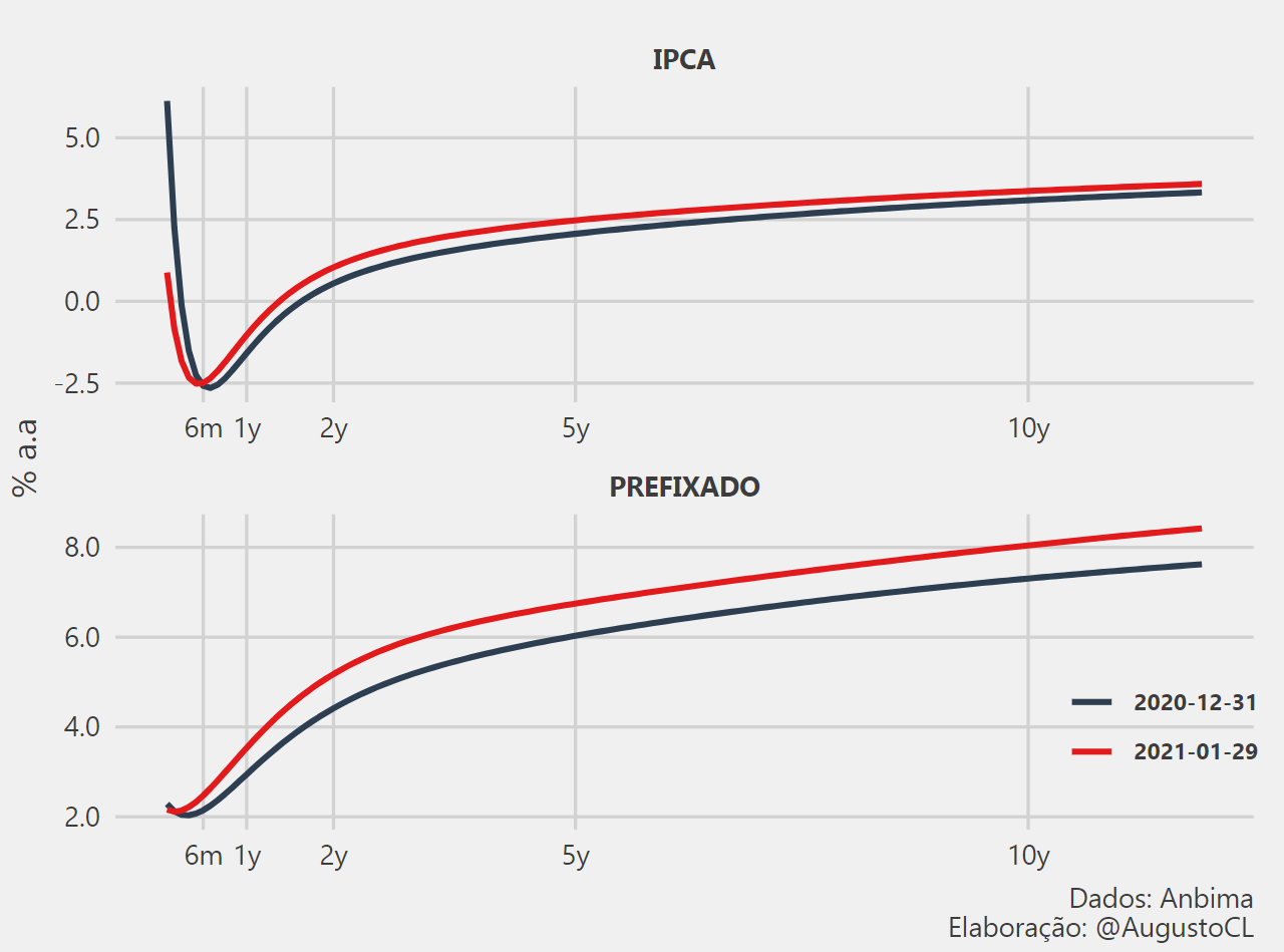
In the next post, I will teach how I created a function that generates this comparative chart from the input of two dates. For now, I have a post on the site with a gif that demonstrates the historical behavior of these yield curves, which can be seen here. The complete code for you to reproduce is also available on github.
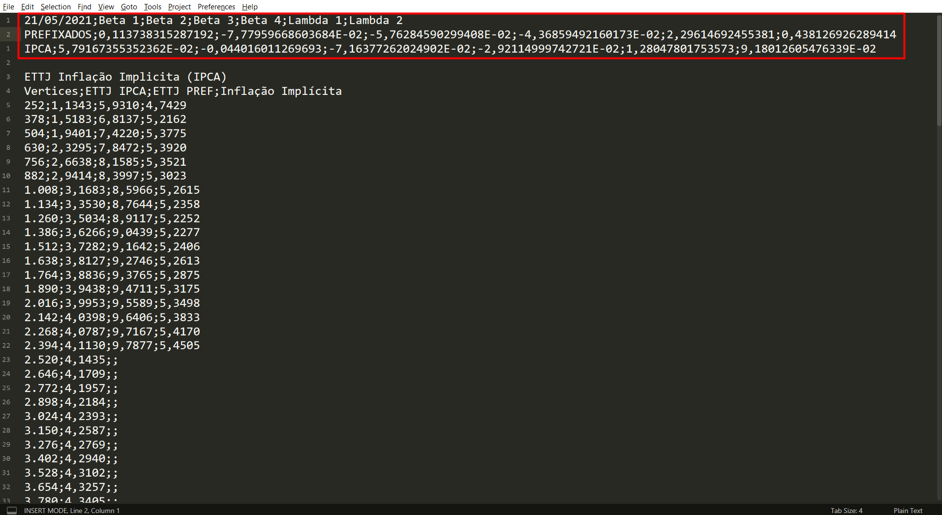
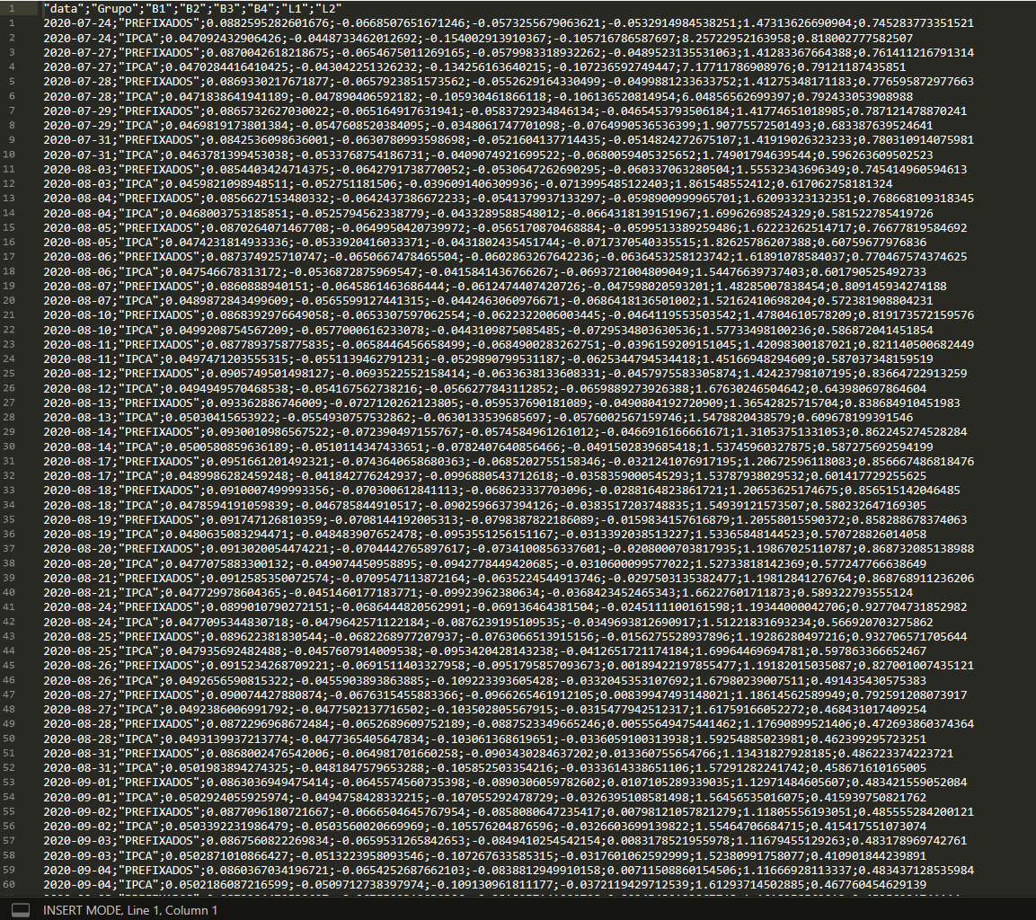
The site allows downloading data in different formats, and in this case, I will use the .csv format. When we open the file in Sublime Text, we observe the following structure in the image below, highlighting the parameters that will be collected.
3 - Creating the R Script
3.1 - Extracting parameters from the ANBIMA website
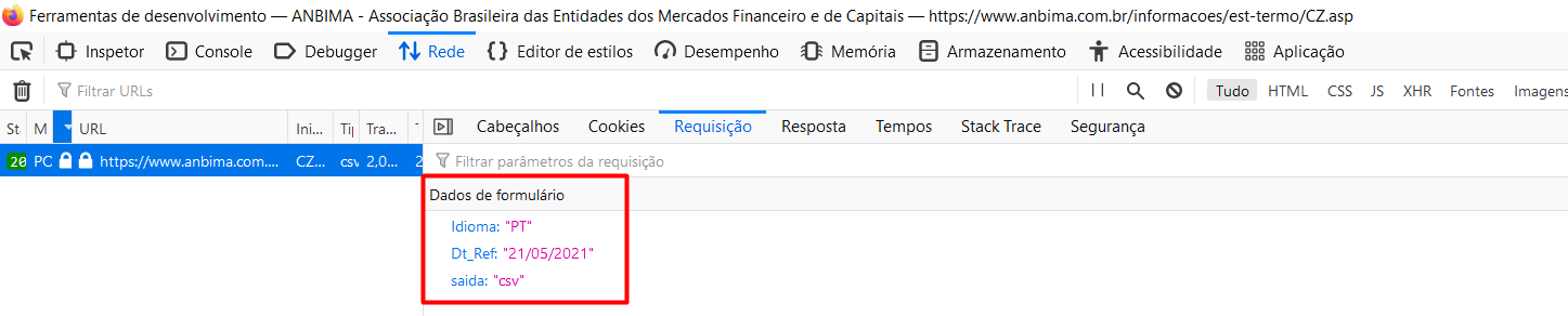
Investigating how the site works when we download data, we can identify, through the browser’s developer tools, a POST request that returns the data in the requested format. Below is an image highlighting the request identification points in the network tab.

When we dig into the request, we find the data that needs to be input for the POST request to return what we want. With this information, we will automate the request via script.
3.2 - Reproducing the request via R script
Now we will go through the request and data cleaning step by step. Then, I will encapsulate everything into a function to iterate this process over the 5 available business days using the purrr package.
With the httr package, it is possible to reproduce the POST request by passing:
- The URL as text in the
urlargument. - A
listobject in thebodyargument with all the request data we saw earlier. - The string “form” for the
encodeargument to identify that the request has a form structure.
url <- "https://www.anbima.com.br/informacoes/est-termo/CZ-down.asp"

dt = "05/06/2026"

r <- httr::POST(url = url,
                body = list(Idioma = "PT",
                            Dt_Ref = dt,
                            saida = "csv"),
                encode = "form")
r
Response [https://www.anbima.com.br/informacoes/est-termo/CZ-down.asp]
Date: 2026-06-06 04:56
Status: 200
Content-Type: text/csv
Size: 3.02 kB
NA3.3 - Cleaning the data
Since the request has status 200, we know it was successful. Now we can check the content with the content() function. With the as argument, the function allows interpreting the result as plain text (‘text’) or binary (‘raw’). From my tests, the best approach is to read the output as binary and then convert it to text using the rawToChar() function.
texto_puro <- iconv(rawToChar(httr::content(r, as = "raw")) , to = "UTF-8", sub = "")With this, we can pass the plain text to the read_csv2() function, which will generate the dataframe with the desired data. Since the text is already configured with scientific notation, the function understands that the data is numeric and interprets it correctly.
But before passing it to the function, remember the image of the .csv file in Sublime Text — we can see that we only need to read the first 3 lines of text (1 header + 2 observations). So we will pass this condition in the n_max argument, adjust the column names, and add a date column. All in a pipe sequence.
dados <-
        read_csv2(texto_puro, n_max = 2) %>%
        `colnames<-`(c("Grupo","B1","B2","B3","B4","L1","L2")) %>%
        mutate(data = dt)

glimpse(dados)
Rows: 2
Columns: 8
$ Grupo <chr> "PREFIXADOS", "IPCA"
$ B1 <dbl> 0.14747611, 0.06977058
$ B2 <dbl> -0.002084683, 0.056084907
$ B3 <dbl> -0.01972741, -0.06848484
$ B4 <dbl> 0.007551824, 0.059301439
$ L1 <dbl> 3.810590, 2.376868
$ L2 <dbl> 0.6918152, 0.5672050
$ data <chr> "05/06/2026", "05/06/2026"3.4 - Encapsulating in a function
Now we can create a function that receives the date and returns our desired dataframe. In this case, we need to generalize the date argument in our code using the format(dt, "%d/%m/%Y") function in the POST request argument and the mutate(data = dt) function in the date column we added to the dataframe. The final function looks like this:
get_ettj_param <- function(dt){

    url <- "https://www.anbima.com.br/informacoes/est-termo/CZ-down.asp"

    r <- httr::POST(url = url,
                    body = list(Idioma = "PT",
                                Dt_Ref = format(dt, "%d/%m/%Y"),
                                saida = "csv"),
                    encode = "form")

    texto_puro <- iconv(rawToChar(httr::content(r, as = "raw")), to = "UTF-8", sub = "")

    dados <-
        read_csv2(texto_puro, n_max = 2) %>%
        `colnames<-`(c("Grupo","B1","B2","B3","B4","L1","L2")) %>%
        mutate(data = dt)

    return(dados)
}
3.5 - Getting the business day vector with bizdays
To iterate over dates, we need to create a vector with the last 5 business days. Fortunately, the bizdays package allows us to select the last 5 business days regardless of when you run the script, considering the official ANBIMA calendar. It is an excellent package.
# load the working days by calendar of anbima
cal <- calendars()[["Brazil/ANBIMA"]]

d2 = Sys.Date()
d1 = add.bizdays(d2, -6, cal = cal)
data_seq <- bizseq(d1, d2, cal)
data_seq
[1] "2026-05-28" "2026-05-29" "2026-06-01" "2026-06-02" "2026-06-03"
[6] "2026-06-05"First, we load the ANBIMA calendar, already available in the package, into the cal variable. Then we get the current date with the Sys.Date() function and the sixth business day back with the add.bizdays(., -6) function, and finally create the vector of the last 5 business days with the bizseq() function.
3.6 - Iterating the function over multiple dates with purrr
purrr allows us to adopt the functional programming paradigm, eliminating for loops from our code by using functions like map(). It also has variations like map_dfr() which, in addition to iterating the input vector over the desired function, also stacks the data, returning a complete data frame.
deal_error <-
    purrr::possibly(get_ettj_param,
                    otherwise = NA_real_) # deal with error
result <-
    purrr::map_dfr(data_seq[1:6], deal_error) %>%
    select(data, everything())

glimpse(result)
Rows: 12
Columns: 8
$ data <date> 2026-05-28, 2026-05-28, 2026-05-29, 2026-05-29, 2026-06-01, 202…
$ Grupo <chr> "PREFIXADOS", "IPCA", "PREFIXADOS", "IPCA", "PREFIXADOS", "IPCA"…
$ B1 <dbl> 0.13932043, 0.06772996, 0.14033783, 0.06766466, 0.14074400, 0.06…
$ B2 <dbl> 0.0041556131, 0.0484948502, 0.0025526762, 0.0482630109, 0.001579…
$ B3 <dbl> -0.02686029, -0.04825871, -0.02086562, -0.04619495, -0.01260969,…
$ B4 <dbl> 0.020513033, 0.040173050, 0.013513644, 0.041425117, 0.009494875,…
$ L1 <dbl> 0.9651316, 2.2285347, 0.9639062, 2.3379521, 0.9608481, 2.3442112…
$ L2 <dbl> 0.3652029, 0.5170365, 0.3647554, 0.5201364, 0.3632370, 0.5200847…In this case, I also use possibly() to handle potential errors in any iteration of the map. With it, if an error occurs in one iteration, it will input NA for the failed data and continue executing the next item without breaking the iteration.
3.7 - Saving the data to a .csv
To finalize the script, we need to create a condition that checks if the .csv file already exists. If it does, it will append the new data to the file; otherwise, it will create a new file with the captured data.
name_db <- "hist_coef_pre_ipca.csv"

if (file.exists(name_db)){
    datas_unicas <- unique(as.Date(read.csv2(name_db,header = 1)$data, "%Y-%m-%d"))

    result <- result %>% filter(!data %in% datas_unicas)

    write.table(result,
                file =  name_db,
                append = TRUE,
                row.names = FALSE,
                col.names = FALSE,
                sep = ";",
                fileEncoding = "UTF-8")
} else {
    write.table(result,
                file =  name_db,
                append = FALSE,
                row.names = FALSE,
                sep = ";",
                fileEncoding = "UTF-8")
}
4 - Scheduling the script execution
With the script ready, we can schedule the scraper execution using a .bat file that runs the R script via command line.
The .bat file looks like this "C:\Program Files\R\R-4.0.2\bin\R.exe" CMD BATCH C:\Users\augus\Documents\dev_R\schedule_R\coef_curv_anbima_scheduler.R
In it, the R executable is passed in the initial string, then the CMD BATCH command calls the command line that will execute the R script that follows.
With this simple code, Windows Task Scheduler will schedule the script execution, and so every week your database will receive the previous week’s data.
To avoid making this post even longer, here is a tutorial on how to schedule tasks with this tool. Just follow these steps and select the .bat file as the program/script to be executed.
For Linux users, you can use
crontabto do the same scheduling. This structure allows running scripts in different languages. For example, if you want to schedule a python script, just use the path to the python executable and reference the .py script you want.
In my case, I schedule the script to run every Monday to capture the data. Since I created the script in July 2020, I have data from that period in my .csv file.
Finally, the R script I use is available in this gist on github. In the next post, I will detail the R script that generates the plot shown at the beginning of the article.