Data Cleaning + Webscraping [R]
This post details the final project for the completion of the Data Cleaning course from Curso-R, where the project required at least:
- Reading a raw dataset that is not in tidy format, where each variable is a column and each row is an observation.
- Manipulating some text column.
- Saving the dataset in tidy format, as a .rds file.
If you want to check the final code without going through the entire step-by-step below, here is the link to the complete script.
TABLE OF CONTENTS
- Case Summary
- Running the Webscraping
- Cleaning the Data (janitor, dplyr, tidyr, stringr)
- Applying Functions with Multiple Dates in a Pipeline (tidyr + purrr)
- Checking the Results
1 - Case Summary
Since I found many public datasets to be relatively clean, I looked for datasets that needed substantial cleaning and thus got excited to perform webscraping to obtain dirty data.
I also took the opportunity to encapsulate the entire process in
purrrfunctions, working with list-columns from the Tidyverse universe. This made the code more readable and reproducible, while also reducing lines of code by avoiding for-loops.
So I captured the energy consumption values in MWh of the 15 largest energy-consuming municipalities in the state of São Paulo, by year, available on the following page of the São Paulo Department of Infrastructure and Environment.
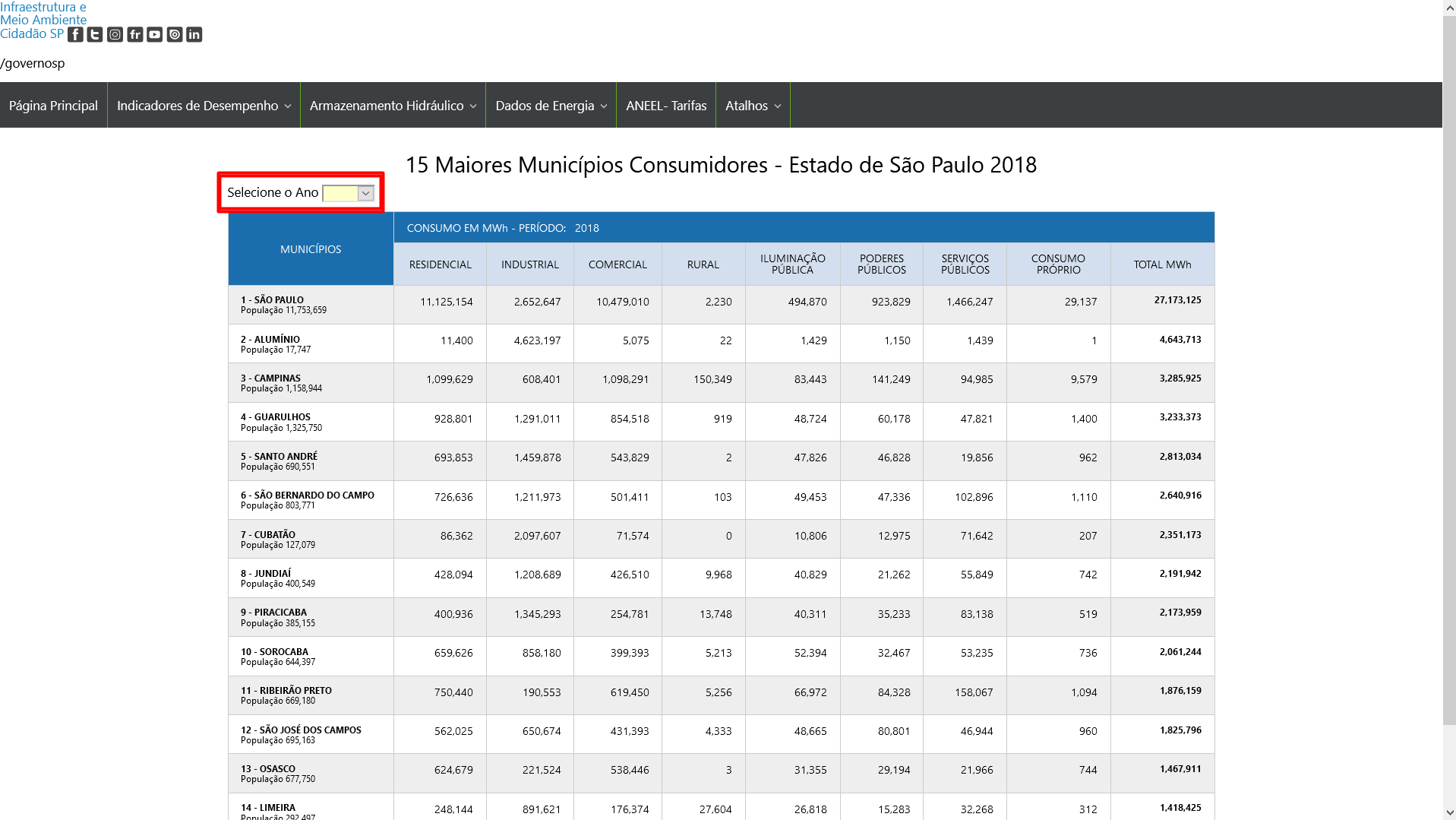
In the red rectangle highlighted in the image, there is a year selection box for this table, which contains data from 2006 to 2019. Therefore, the complete dataset has about 210 observations (14x15).
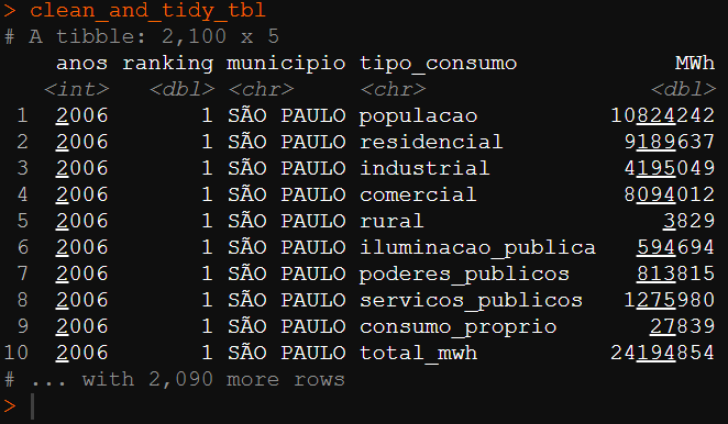
This dataset can be considered untidy because we have several columns representing the same type of consumption information. So to transform the dataset into tidy format, these columns need to be turned into a single variable called “consumption_type”.
1.1 - Dirty Untidy Dataset
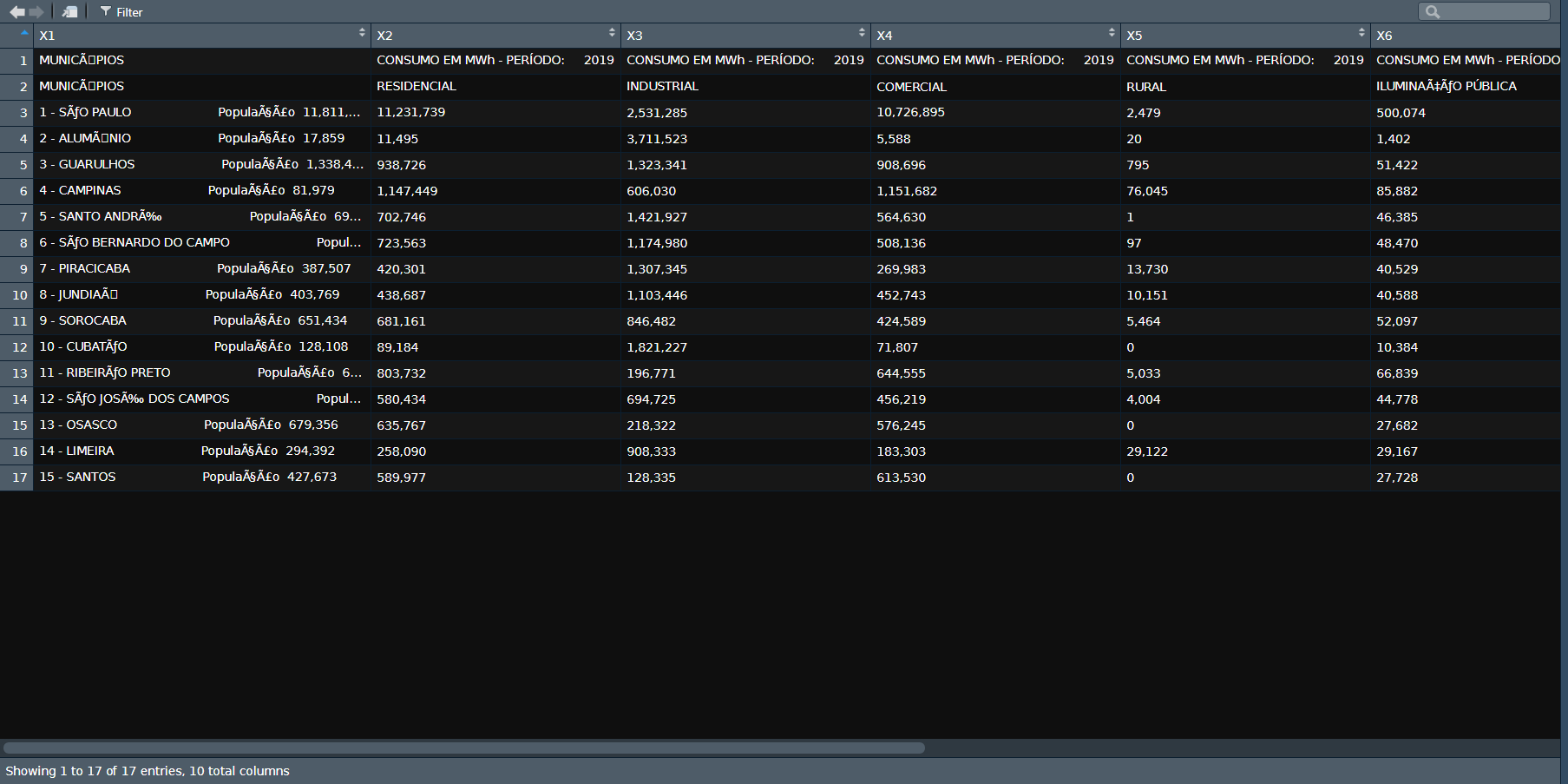
The raw webscraping extraction generates the following dirty dataset with encoding issues.
1.2 - Clean Tidy Dataset
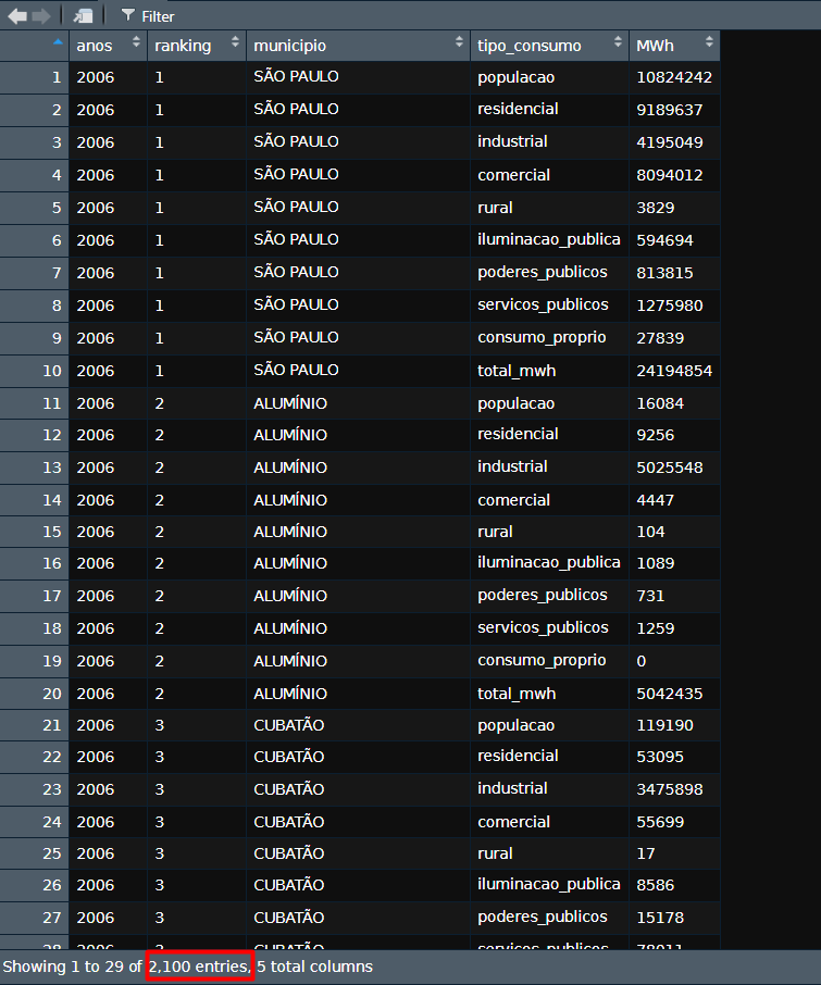
After webscraping, cleaning, and data treatment, we obtain the following final dataset in the requested tidy format.
2 - Running the Webscraping
2.1 - Identifying the request on the site
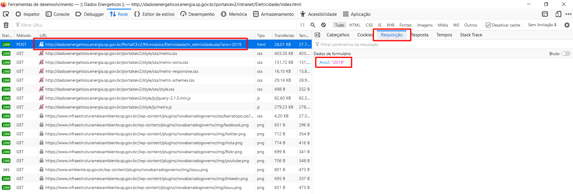
When we open the network section of the browser's developer tools and select a new year in the table, we can identify the POST request that returns the HTML of the page containing the table.
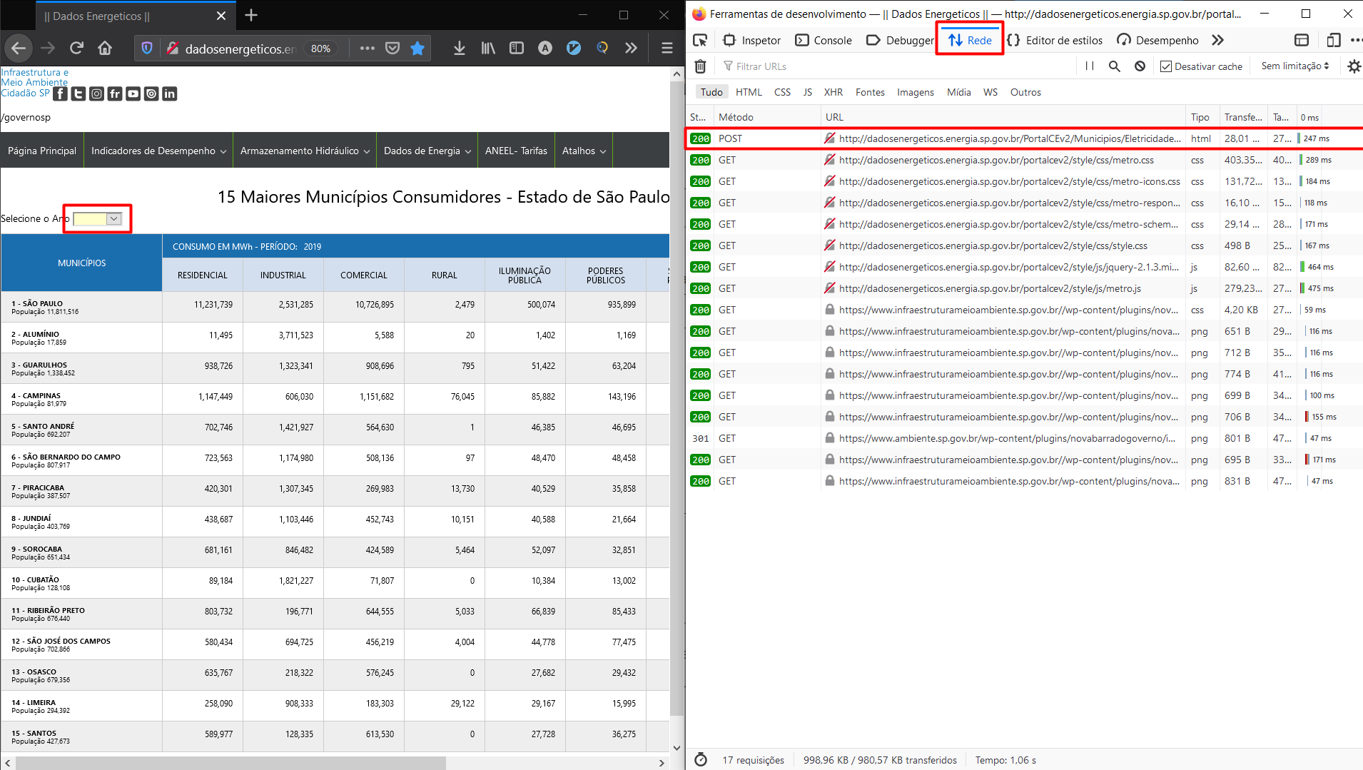
By investigating this request, we can extract the requested URL and the necessary form fields.
2.2 - Recreating the request via script (httr, rvest, stringr)
With the information in hand, we can reproduce the same request via code as follows.
aaaa <- 2019
url <- "http://dadosenergeticos.energia.sp.gov.br/PortalCEv2/Municipios/Eletricidade/m_eletricidade.asp?ano={aaaa}"
req <- httr::POST(url = glue::glue(url),
                  body = list(Ano2 = aaaa),
                  encode = "form")
The result is a list with several pieces of request information, where the main content is in binary format. So we use the rawToChar() function to convert the binary data to text, thus obtaining the full page HTML.
raw_html <- rawToChar(req$content)Inside the HTML there is a <table> tag that contains all the data we need, but we need to select only the text of this tag to proceed with reading the table. For this, I applied a regex expression that selects all text between the <table and </table> tags in the gsub() function. Then, I prepended the string <table which was not captured by the previous function. This way, we obtain an HTML string that is recognized as a table by the html_table() function.
text_inside_html_table <-
  gsub('^.*<table\\s*|\\s* <\\/table>*$', '', raw_html) %>%
  paste0("<table ", .)
Then I applied the read_html() and html_table() functions from the rvest package, extracted the table with pluck(), and converted it to a dataframe, resulting in the dirty table presented in the problem introduction.
dirty_tibble <- text_inside_html_table %>%
  rvest::read_html() %>%
  rvest::html_table() %>%
  purrr::pluck() %>%
  base::as.data.frame() %>%
  dplyr::as_tibble()

glimpse(dirty_tibble)
## Rows: 17
## Columns: 10
## $ X1 <chr> "MUNICÃ\u008dPIOS", "MUNICÃ\u008dPIOS", "1 - SÃO PAULO\r\n ~
## $ X2 <chr> "CONSUMO EM MWh - PERÍODO: 2019", "RESIDENCIAL", "11,231,739",~
## $ X3 <chr> "CONSUMO EM MWh - PERÍODO: 2019", "INDUSTRIAL", "2,531,285", "~
## $ X4 <chr> "CONSUMO EM MWh - PERÍODO: 2019", "COMERCIAL", "10,726,895", "~
## $ X5 <chr> "CONSUMO EM MWh - PERÍODO: 2019", "RURAL", "2,479", "20", "795~
## $ X6 <chr> "CONSUMO EM MWh - PERÍODO: 2019", "ILUMINAÇÃO PÚBLICA", "500~
## $ X7 <chr> "CONSUMO EM MWh - PERÍODO: 2019", "PODERES PÚBLICOS", "935,899~
## $ X8 <chr> "CONSUMO EM MWh - PERÍODO: 2019", "SERVIÇOS PÚBLICOS", "1,554,~
## $ X9 <chr> "CONSUMO EM MWh - PERÍODO: 2019", "CONSUMO PRÓPRIO", "28,905",~
## $ X10 <chr> "CONSUMO EM MWh - PERÍODO: 2019", "TOTAL MWh", "27,511,918", "~2.3 - Solving encoding issues (stringr)
Looking at the HTML text of the raw_html variable, I noticed these encoding issues. I used the guess_encoding() function and found the encoding was the classic UTF-8. I tried different encoding conversion functions I found online, but none worked. Since there were only a few cases, I decided to do manual substitutions and added this cleaning to the code as follows.
raw_html <- rawToChar(req$content) %>%
  str_replace_all(., "Ã\u008d", "Í") %>%
  str_replace_all(., "ÇÃ", "ÇÃ") %>%
  str_replace_all(., "Ã", "Ã") %>%
  str_replace_all(., "É", "É") %>%
  str_replace_all(., "çã", "çã")
3 - Cleaning the Data (janitor, dplyr, tidyr, stringr)
So far we have the following dirty and untidy table.
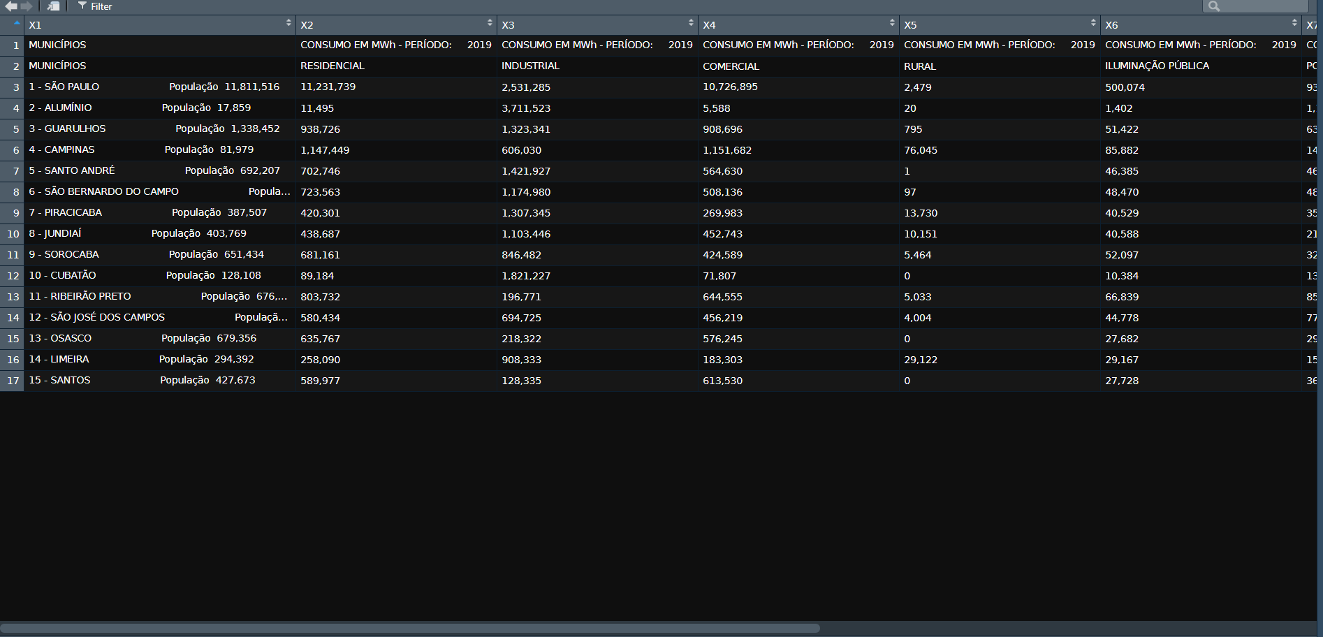
Proceeding, I removed the first row which contains repeated and unnecessary information, turned the second row into column names, and applied name cleaning with the clean_names() function from the janitor package.
consumo_2019 <- scrapy_consumo_eletr_ano(2019)

consumo_2019 %>%
  slice(-1) %>%
  janitor::row_to_names(row_number = 1) %>%
  janitor::clean_names() %>%
  rename(total_mwh = total_m_wh) %>%
  glimpse()
## Rows: 15
## Columns: 10
## $ municipios <chr> "1 - SÃO PAULO\r\n \r\n Populaçã~
## $ residencial <chr> "11,231,739", "11,495", "938,726", "1,147,449", "70~
## $ industrial <chr> "2,531,285", "3,711,523", "1,323,341", "606,030", "~
## $ comercial <chr> "10,726,895", "5,588", "908,696", "1,151,682", "564~
## $ rural <chr> "2,479", "20", "795", "76,045", "1", "97", "13,730"~
## $ iluminacao_publica <chr> "500,074", "1,402", "51,422", "85,882", "46,385", "~
## $ poderes_publicos <chr> "935,899", "1,169", "63,204", "143,196", "46,695", ~
## $ servicos_publicos <chr> "1,554,641", "1,457", "77,472", "95,976", "20,061",~
## $ consumo_proprio <chr> "28,905", "0", "1,195", "9,724", "963", "1,097", "5~
## $ total_mwh <chr> "27,511,918", "3,732,654", "3,364,850", "3,315,985"~Since the municipio variable also contains ranking and population information, I applied the separate() function twice to transform the variable into 3 columns (ranking, municipio, and populacao). For this, I used the strings " - " and “População” as separators, as shown in the code below.
  ... %>%
  separate(col = "municipios",
           sep = "População",
           into = c("municipio", "populacao")) %>%
  separate(col = "municipio",
           sep = " - ",
           into = c("ranking", "municipio")) %>%
After the separations, we have the following dataset.
## Rows: 15
## Columns: 12
## $ ranking            <chr> "1", "2", "3", "4", "5", "6", "7", "8", "9", "10", ~
## $ municipio          <chr> "SÃO PAULO\r\n           \r\n          ", "ALUMÍNIO~
## $ populacao          <chr> "  11,811,516", "  17,859", "  1,338,452", "  81,97~
## $ residencial        <chr> "11,231,739", "11,495", "938,726", "1,147,449", "70~
## $ industrial         <chr> "2,531,285", "3,711,523", "1,323,341", "606,030", "~
## $ comercial          <chr> "10,726,895", "5,588", "908,696", "1,151,682", "564~
## $ rural              <chr> "2,479", "20", "795", "76,045", "1", "97", "13,730"~
## $ iluminacao_publica <chr> "500,074", "1,402", "51,422", "85,882", "46,385", "~
## $ poderes_publicos   <chr> "935,899", "1,169", "63,204", "143,196", "46,695", ~
## $ servicos_publicos  <chr> "1,554,641", "1,457", "77,472", "95,976", "20,061",~
## $ consumo_proprio    <chr> "28,905", "0", "1,195", "9,724", "963", "1,097", "5~
## $ total_mwh          <chr> "27,511,918", "3,732,654", "3,364,850", "3,315,985"~
Next, I removed line breaks and extra spaces with the str_squish() function from the stringr package, which removes all such dirt from both the beginning and end of the text. Then I removed commas from the value variables and finally converted these variables to numeric types.
.... %>%
  mutate(
  across(ranking:populacao,
         ~str_squish(.)),
  across(c(ranking, populacao:total_mwh),
         ~as.numeric(str_replace_all(., ",", "")))
  )
4 - Applying Functions with Multiple Dates in a Pipeline (tidyr + purrr)
Aiming to allow visualization of the work steps in list-column tables, I separated the data extraction and cleaning into two functions called:
- scrapy_consumo_eletr_ano()
- clean_table()
scrapy_consumo_eletr_ano <- function(ano){

    # requisicao POST
    aaaa <- ano
    url <- "http://dadosenergeticos.energia.sp.gov.br/PortalCEv2/Municipios/Eletricidade/m_eletricidade.asp?ano={aaaa}"
    req <- httr::POST(url = glue::glue(url),
                      body = list(Ano2 = aaaa),
                      encode = "form")

    # converte o binario do html para string
    raw_html <- rawToChar(req$content) %>%
      str_replace_all(., "Ã\u008d", "Í") %>%
      str_replace_all(., "ÇÃ", "ÇÃ") %>%
      str_replace_all(., "Ã", "Ã") %>%
      str_replace_all(., "É", "É") %>%
      str_replace_all(., "çã", "çã")

    # usando regex, extrai o bloco de código equivalente a tabela do html
    text_inside_html_table <-
        gsub('^.*<table\\s*|\\s* <\\/table>*$', '', raw_html) %>%
        paste0("<table ", .)

    # converte o html da tabela em dataframe
    dirty_tibble <- text_inside_html_table %>%
        read_html() %>%
        html_table() %>%
        pluck() %>%
        as.data.frame() %>%
        as_tibble()
}

# Função de Limpeza da Base -----------------------------------------------

clean_table <- function(tbl){

  tbl %>%
    slice(-1) %>%
    janitor::row_to_names(row_number = 1) %>%
    janitor::clean_names() %>%
    rename(total_mwh = total_m_wh) %>%
    separate(col = "municipios",
             sep = "População",
             into = c("municipio", "populacao")) %>%
    separate(col = "municipio",
             sep = " - ",
             into = c("ranking", "municipio")) %>%
    mutate(
      across(ranking:populacao,
             ~str_squish(.)),
      across(c(ranking, populacao:total_mwh),
             ~as.numeric(str_replace_all(., ",", "")))
      )
}
This way, it was possible to run the iterations with the map() function from purrr and save all results and intermediate steps in a single aggregating table called all_tbl.
all_tbl <-
  list("anos" = c(2006:2019)) %>%
  as_tibble() %>%
  mutate(
    raw_tbl = purrr::map(anos,
                         scrapy_consumo_eletr_ano),
    clean_but_not_tidy_tbl = purrr::map(raw_tbl,
                                        clean_table),
    clean_and_tidy_tbl = purrr::map(clean_but_not_tidy_tbl,
                                    ~unnest(.) %>%
                                      pivot_longer(populacao:total_mwh,
                                                   names_to = "tipo_consumo",
                                                   values_to = "MWh")
                                    )
    )
If you are not familiar with tidyr's list-column structure, I suggest checking out this chapter from the Curso-R book at this link.
I could have applied the pivot_longer() function in the cleaning function, returning the dataset already in tidy format. However, since I want to demonstrate the different phases of treatment using purrr, I preferred to recreate an anonymous function inside the map. This way the reader experiences different approaches to the tool.
5.0 - Checking the Results
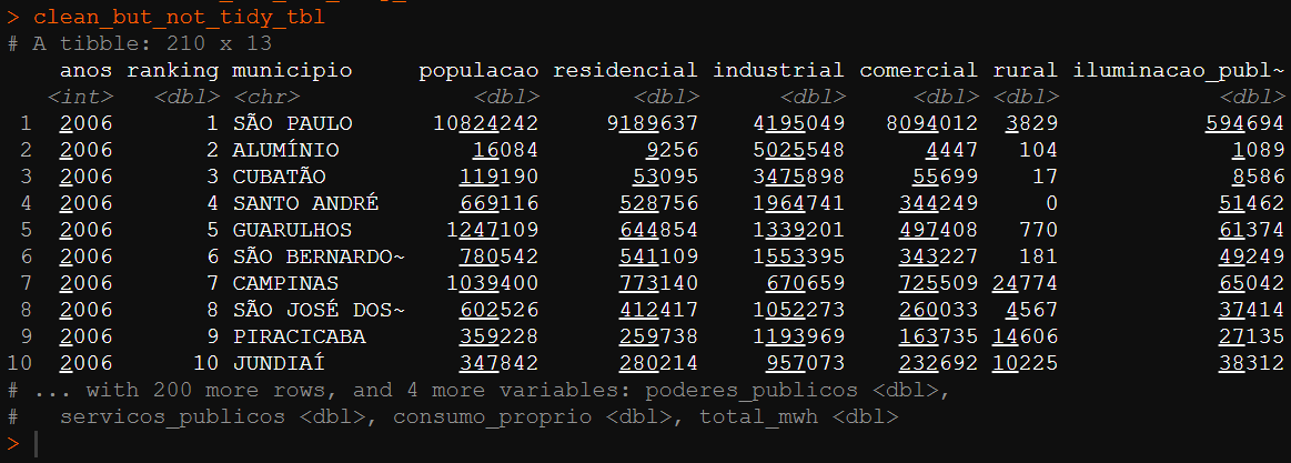
The all_tbl object has the following structure with tables in column-list format.
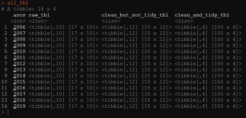
To extract each of the intermediate and result tables, I used the unnest() function as follows.
# dados brutos
raw_tbl <-
  all_tbl %>%
  select(anos, raw_tbl) %>%
  unnest(raw_tbl)

# dados limpos, mas não tidy
clean_but_not_tidy_tbl <-
  all_tbl %>%
  select(anos, clean_but_not_tidy_tbl) %>%
  unnest(clean_but_not_tidy_tbl)

# dados limpos e tidy
clean_and_tidy_tbl <-
  all_tbl %>%
  select(anos, clean_and_tidy_tbl) %>%
  unnest(clean_and_tidy_tbl)
This way, we can check the 3 phases of the work: raw data, clean but untidy data, and clean and tidy data.
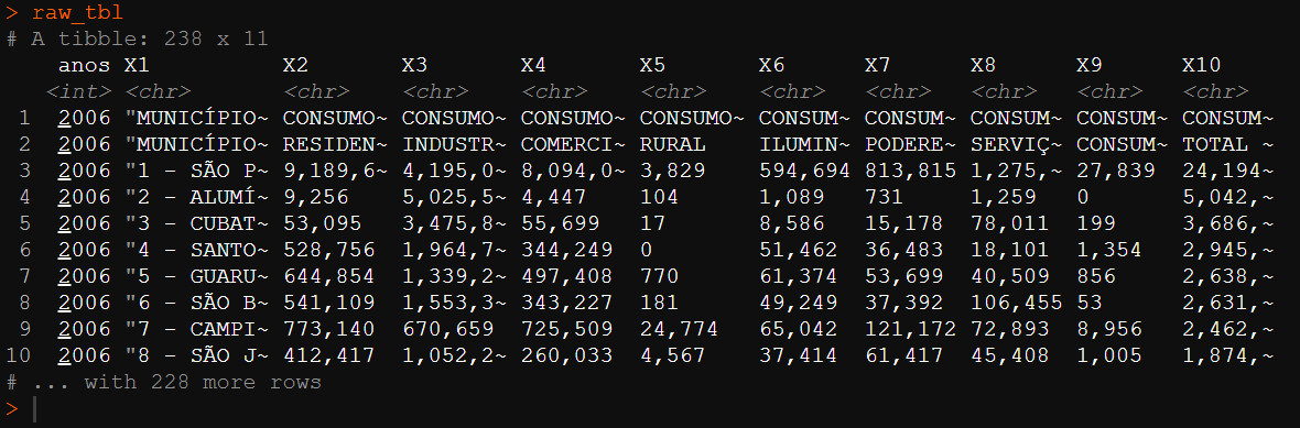
Finally, I saved the results in .rds format, as requested by the activity.
write_rds("clean_and_tidy_tbl", clean_and_tidy_tbl)